Electron Orbital Visualization
This notebook was developed for the Quantum Chemistry graduate course (CHM 6470 - Chemical Bonding and Spectra I) at the University of Florida. It used the Hydrogen atom wavefunctions to provide visualizations of the quantum equations of the atomic orbitals. The visualization requires the use of the "mayavi2" library to display isoplots (surfaces of equal value) of the probability density functions. It is these functions that can be interpreted as describing the most probable location for finding an electron.
Usage:
To use this notebook start it with the following command:
ipython notebook
Authors:
- Damon Allen Ph.D.
- Nick Polfer Ph.D.
- Corey Stedwell Ph.D. Candidate
Debugging help from:
- Nathan Roehr Ph.D. Candidate
Acknowledgements
This project is financially supported by the National Science Foundation under grant CHE-0845450.
The information in this notebook is partially based on the information found at the following sites:
http://panda.unm.edu/Courses/Finley/P262/Hydrogen/WaveFcns.html
http://www.hasenkopf2000.net/wiki/page/3d-hydrogen-structure-python/
Sample output using quantum number values of $n=3$, $l=2$, $m=0$

- Number of contours used = 16
- Opacity = 0.5
Quantum Equations
The (radial) probability function can be expressed as the product of the square of the wavefunction ($\psi$) times the square of the distance (r) from the nucleus.
$P = \psi^2 r^2$ (probability function)
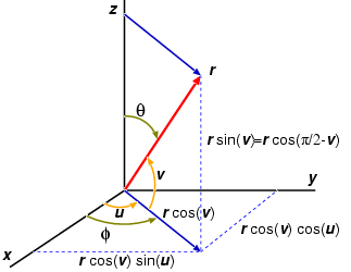
$\psi$ is a wavefunction that is composed of the radial ($R_{nl}$) and the spherical harmonics ($Y_{lm}$) functions. $R_{nl}$ is dependent on the distance from the center of the atom $r$, and the principal quantum number $n$, and angular momentum quantum number $l$. $Y_{lm}$ is a function of $l$, the magnetic angular momentum $m_l$, $\phi$ (defined as the angle of the positon vector in the $\textbf{xy}$ plane), and $\theta$ (i.e., angle between $\textbf{z}$-axis and position vector) in a spherical coordinate system. For the purposes of this notebook $m_l$ will be expressed simply by the term $m$ to avoid confusion with $l$.
 $$\psi_{nlm}(r,\theta,\phi) = R_{nl}(r)Y_{lm}(\theta,\phi)$$
(Note: In the following derivations for $\psi$, $R$ and $Y$'s the quantum number subscripts are dropped in order to prevent confusion with multiplication terms.)
Where:
$$R(r) = \left(\frac{2\cdot z}{n\cdot a_0}\right)^{3/2} \sqrt{\frac{(n-l-1)!}{2\cdot n\cdot [(n+l)!]^3}}\cdot exp\left(\frac{-z\cdot r}{n \cdot a_0}\right) \cdot \left(\frac{2\cdot z\cdot r}{n \cdot a_0} \right)^l \cdot L^{2\cdot l +1}_{n-l-1} \left(\frac{2 \cdot z \cdot r}{n\cdot a_0} \right)$$Where:
$z$ refers to the atomic charge of the nucleus (i.e., +1 for hydrogen)
$a_0$ refers to the Bohr radius (assume $a_0 = 1$ for unity)
and $L$ is a Laguerre polynomial:
$$\hspace{20 mm}\text{Where: } L^{2\cdot l +1}_{n-l-1}\left(\frac{2 \cdot z \cdot r}{n\cdot a_0} \right) = \sum_{i=0}^{n-l-1}{\frac{(-i)^i\cdot\left((n+l)!\right)^2 \left( \frac {2zr}{n a_0}\right)^i} {i!\cdot(n-l-1-i)!\cdot(2\cdot l+1+i)!}}$$Where $P_l^m$ is a Legendre polynomial.
$$\hspace{20 mm}\text{Where: }P^{|m|}_{l}(cos(\theta))=\left(1-cos^2(\theta)\right)^{\left|\frac{m}{2}\right|} \cdot \frac{\delta^{|m|} }{\delta (cos(\theta))^{|m|}}(P_l(cos(\theta)))$$$$\hspace{20 mm}\text{Where: }P^{|m|}_{l}(cos(\theta))=sin^{\left|m\right|}(\theta) \cdot \frac{\delta^{|m|} }{\delta (cos(\theta))^{|m|}}(P_l(cos(\theta)))$$$\hspace{20 mm}$Rodrigues’ formula provides a solution to the Legendre polynomial $P_l$.
$$\hspace{20 mm}\hspace{20 mm}\text{and where: }P_l(cos(\theta)) = \frac{1}{2^l\cdot l!} \frac{d^l}{d (cos(\theta))^l} (cos^2(\theta)-1)^l$$(Note that the $\delta^m$ term refers refers to the derivative with order m with respect to $cos(\theta)$ and the $d^l$ term refers to the derivative with order $l$ with respect to $cos(\theta)$.)
Displaying the Orbitals
For purposes of display we are only intrested in the real portion of $Y^{m}_{l}(\theta,\phi)$.
Specifically, if $m\ne0$ then we evaluate $Y$ in with the following modifications.
For the real part:
$$Y^{m}_{l}(\theta,\phi)=\left|\sqrt{\frac{(2\cdot l+1)(l-|m|)!}{4\cdot\pi\cdot (l+|m|)!}}\cdot \left(\sqrt{2} \cdot \Re\left\{e^{i\cdot m \cdot\phi}\right\}\right)\cdot P^{|m|}_{l}(cos(\theta))\right|$$(If $m>0$)
(Note that the $(-1)^{|m|}$ goes away when only using the real or imaginary portions but you have to take the absolute value.)
(Note that $\Re\left\{e^{i\cdot m \cdot\phi}\right\}$ denotes the real part of $e^{i\cdot m \cdot\phi}$)
or, for the imaginary part:
$$Y^{m}_{l}(\theta,\phi)=\left|\sqrt{\frac{(2\cdot l+1)(l-|m|)!}{4\cdot\pi\cdot (l+|m|)!}}\cdot \left(\sqrt{2} \cdot \Im\left\{e^{i\cdot m \cdot\phi}\right\}\right)\cdot P^{|m|}_{l}(cos(\theta))\right|$$(If $m<0$)
(Note that the real and imaginary portions are multiplied with a scaling factor equal to $\frac{2}{\sqrt{2}} = \sqrt{2}$)
Notes on computational alternatives:
When solving the real or imaginary portions by hand the Euler's formula is used and the results are added up.
For example, if $l=1$ and $m=1$, the real solution is:
$=\frac{1}{2}\cdot\sqrt{\frac{3}{2\cdot\pi}}\cdot sin(\theta)\cdot\left(cos(\phi)-i\cdot sin(\phi) + cos(\phi)+i\cdot sin(\phi) \right)$
$=\frac{1}{2}\cdot\sqrt{\frac{3}{2\cdot\pi}}\cdot sin(\theta)\cdot\left(cos(\phi) + cos(\phi) \right)$
$=\frac{1}{2}\cdot\sqrt{\frac{3}{2\cdot\pi}}\cdot sin(\theta)\cdot 2 \cdot cos(\phi) $
$=\sqrt{\frac{3}{2\cdot\pi}}\cdot sin(\theta)\cdot cos(\phi) $
This result needs to be scaled scaling by a factor $\frac{1}{\sqrt{2}}$.
$=\frac{1}{\sqrt{2}}\cdot\sqrt{\frac{3}{2\cdot\pi}}\cdot sin(\theta)\cdot cos(\phi) $
$=\sqrt{\frac{3}{4\cdot\pi}}\cdot sin(\theta)\cdot cos(\phi) $
Import Libraries:
In order to have mayavi.mlab display correctly, version 2.7 of Python must be used.
import sys #texting for the right version of Python to use with mayavi
print("Python version = {}".format(sys.version))
print("Machine readable Python version = {}".format(sys.version_info))
sys.version_info[0]
Python version = 2.7.5+ (default, Sep 19 2013, 13:48:49)
[GCC 4.8.1]
Machine readable Python version = sys.version_info(major=2, minor=7, micro=5, releaselevel='final', serial=0)
2
Additionally, this notebook uses the sympy library to symbolically develop the equations needed to calculate the probability function to the wave equation. Once derived these equations are converted to numpy versions for speed and compatibility with the mayavi library.
(Note: To install mayavi2 on Ubuntu 12.04, type "sudo apt-get install mayavi2" in the terminal window.)
print("The library version numbers used in this notebook are:")
if sys.version_info[0]==2:
    #this requires the use of no higher than python 2.7
    from mayavi import __version__ as mayavi_version
#     import scipy.special
#     import scipy.misc
    from mayavi import mlab
    print("mayavi version:  %s"%mayavi_version)
else:
    print("The use of mayavi.mlab to display the orbital requires the "+\
          "use of Python 2.7.3")

from IPython import __version__ as IPython_version
from IPython.display import Latex
import numpy as np
import sympy

#"I" is sympy's imaginary number
from sympy import symbols,I,latex,pi,diff
from sympy.utilities.lambdify import lambdastr
from sympy import factorial as fac
from sympy.functions import Abs,sqrt,exp,cos,sin
from sympy import re, im, simplify

#display the latex representation of a symbolic variable by default.
from sympy import init_printing
init_printing(use_unicode=True)

a_0,z,r=symbols("a_0,z,r")
n,m,l=symbols("n,m,l",integer=True)
int_m=symbols("int_m",integer=True)
theta,phi = symbols("\\theta,\\phi",real=True)

#The variables will used with lambdify...
angle_theta, angle_phi, radius = symbols("angle_theta,angle_phi,radius",
                                         real=True)


print("numpy version:   %s"%np.__version__)
print("sympy version:   %s"%sympy.__version__)

print("IPython version: %s"%IPython_version)
The library version numbers used in this notebook are:
mayavi version:  4.1.0
numpy version:   1.7.1
sympy version:   0.7.4.1
IPython version: 1.2.0
(Note: Even though the SciPy library has both the Laguerre and and spherical harmonics functions in it, for purposes of clarity in the derivation and consistency in the way orbitals have been traditionally represented in Chemistry, specific solutions of these functions are developed and written here.)
Declare Functions:
Defining $P_l$ (Legendre polynomial):
def P_l(l,theta): #valid for l greater than equal to zero
    """Legendre polynomial"""
    if l>=0:
        eq=diff((cos(theta)**2-1)**l,cos(theta),l)
    else:
        print("l must be an integer equal to 0 or greater")
        raise ValueError
    return 1/(2**l*fac(l))*eq
Validation
P_l(0,theta)
P_l(1,theta)
P_l(2,theta)
Defining $P^{|m|}_{l}$ (Legendre polynomial):
Which equals...
$$P^{|m|}_{l}(cos(\theta))=sin^{\left|m\right|}(\theta) \cdot {\frac{\delta^{|m|} }{\delta (cos(\theta))^{|m|}}(P_l(cos(\theta)))}$$def P_l_m(m,l,theta):
"""Legendre polynomial"""
eq = diff(P_l(l,theta),cos(theta),Abs(m))
result = sin(theta)**Abs(m)*eq #note 1-cos^2(theta) = sin^2(theta)
return result
Validation
P_l_m(1,1,theta) #Because sqrt(1-cos^(theta)) = sin(theta)
P_l_m(-1,1,theta)
Defining $Y^{m}_{l}(\theta,\phi)$ (Spherical harmonics):
(If $m>0$)
or
$$Y^{m}_{l}(\theta,\phi)=\left|\sqrt{\frac{(2\cdot l+1)(l-|m|)!}{4\cdot\pi\cdot (l+|m|)!}}\cdot \left(\sqrt{2} \cdot \Im\left\{e^{i\cdot m \cdot\phi}\right\}\right)\cdot P^{|m|}_{l}(cos(\theta))\right|$$(If $m<0$)
def Y_l_m(l,m,phi,theta):
    """Spherical harmonics"""
    eq = P_l_m(m,l,theta)
    if m>0:
        pe=re(exp(I*m*phi))*sqrt(2)
    elif m<0:
        pe=im(exp(I*m*phi))*sqrt(2)
    elif m==0:
        pe=1
    return abs(sqrt(((2*l+1)*fac(l-Abs(m)))/(4*pi*fac(l+Abs(m))))*pe*eq)
Validation
Y_l_m(0,0,phi,theta)
Y_l_m(1,0,phi,theta)
l=1
m=-1
Y_l_m(l,m,phi,theta)
l=1
m=1
Y_l_m(l,m,phi,theta)
print(Y_l_m(1,1,phi,theta)) #showing the computer's version of symbolic
sqrt(3)*Abs(sin(\theta)*cos(\phi))/(2*sqrt(pi))
Defining L, R, $\psi$, and the probability function P:
def L(l,n,rho):
    """Laguerre polynomial"""
    _L = 0.
    for i in range((n-l-1)+1): #using a loop to do the summation
        _L += ((-i)**i*fac(n+l)**2.*rho**i)/(fac(i)*fac(n-l-1.-i)*\
                                          fac(2.*l+1.+i))
    return _L

def R(r,n,l,z=1.,a_0=1.):
    """Radial function"""
    rho = 2.*z*r/(n*a_0)
    _L = L(l,n,rho)
    _R = (2.*z/(n*a_0))**(3./2.)*sqrt(fac(n-l-1.)/\
         (2.*n*fac(n+l)**3.))*exp(-z/(n*a_0)*r)*rho**l*_L
    return _R
def Psi(r,n,l,m,phi,theta,z=1,a_0=1):
    """Wavefunction"""
    _Y = Y_l_m(l,m,phi,theta)
    _R = R(r,n,l)
    return _R*_Y

def P(r,n,l,m,phi,theta):
    """Returns the symbolic equation probability of the location
    of an electron"""
    return Psi(r,n,l,m,phi,theta)**2*r**2
Orbital Plotting Functions
r_fun = lambda _x,_y,_z: (np.sqrt(_x**2+_y**2+_z**2))
theta_fun = lambda _x,_y,_z: (np.arccos(_z/r_fun(_x,_y,_z)))
phi_fun = lambda _x,_y,_z: (np.arctan(_y/_x)*(1+_z-_z))

def display_orbital(n,l,m_,no_of_contours = 16,Opaque=0.5):
    """Diplays a 3D view of electron orbitals"""
    #The plot density settings (don't mess with unless you are sure)
    rng = 12*n*1.5 #This determines the size of the box
    _steps = 55j#           (it needs to be bigger with n).
    _x,_y,_z = np.ogrid[-rng:rng:_steps,-rng:rng:_steps,-rng:rng:_steps]

    #Plot tweaks
    color = (0,1.0,1.0) #relative RGB color (0-1.0 vs 0-255)
    mlab.figure(bgcolor=color) #set the background color of the plot


    P_tex = "" #initialize the LaTex string of the probabilities

    #Validate the quantum numbers
    assert(n>=1), "n must be greater or equal to 1"       #validate the value of n
    assert(0<=l<=n-1), "l must be between 0 and n-1"      #validate the value of l
    assert(-l<=max(m_)<=l), "p must be between -l and l"  #validate the value of p
    assert(-l<=min(m_)<=l), "p must be between -l and l"  #validate the value of p


    for m in m_:
        #Determine the probability equation symbolically and convert
        #it to a string
        prob = lambdastr((radius,angle_phi,angle_theta), P(radius,n,l,m,
                                                           angle_phi,
                                                           angle_theta))

        #record the probability equation as a LaTex string
        P_eq = simplify(P(r,n,l,m,phi,theta))
        P_tex+="$$P ="+latex(P_eq)+"$$ \n\n "


        #print("prob before substitution = \n\n".format(prob)) #for debugging

        if '(nan)' in prob: #Check for errors in the equation
            print("There is a problem with the probability function.")
            raise ValueError

        #Convert the finctions in the probability equation from the sympy
        #library to the numpy library to allow for the use of matrix
        #calculations
        prob = prob.replace('sin','np.sin') #convert to numpy
        prob = prob.replace('cos','np.cos') #convert to numpy
        prob = prob.replace('Abs','np.abs') #convert to numpy
        prob = prob.replace('pi','np.pi')   #convert to numpy
        prob = prob.replace('exp','np.exp') #convert to numpy

        #print("prob after substitution = \n\n".format(prob)) #for debugging

        #convert the converted string to a callable function
        Prob = eval(prob)

        #generate a set of data to plot the contours of.
        w = Prob(r_fun(_x,_y,_z),phi_fun(_x,_y,_z),theta_fun(_x,_y,_z))

        #add the generated data to the plot
        mlab.contour3d(w,contours=no_of_contours,opacity = Opaque, transparent=True)

    mlab.colorbar()
    mlab.outline()
    mlab.show() #this pops up a interactive window that allows you to
    #            rotate the view


    #Information used for the 2D slices below
    limits = []
    lengths = []
    for cor in (_x,_y,_z):
        limit = (np.min(cor),np.max(cor))
        limits.append(limit)
        #print(np.size(cor))
        lengths.append(np.size(cor))
        #print(limit)
    return (limits, lengths, _x, _y, _z, P_tex)
Displaying the Orbitals:
To display the orbital(s), execute the cell below .
Notes on the quantum numbers:
- $n$ is greater than or equal to 1
- $l$ falls within the inclusive range of zero to $n - 1$
- $m$ is within the range of negative $l$ to positive $l$
#    Set the quantum numbers for the orbitals (all in one spot)
import warnings # in order to suppress divide_by_zero warnings...

print("n must be greater or equal to 1.")
n = int(raw_input("Entry the quantum number for n = "))

print("")
l_str = raw_input("Enter a value for l such that it is less than n (default l=n-1) l = ")
if l_str=="":
    l=n-1
else:
    l = int(l_str)

print("\nThe next value, m, determines which specific orbital will be displayed.")
print("Enter a value(s) for m such that -l <= m <= l.\n"+\
      "m can be a single number for a single orbital or a range for multiple.")
m_str = raw_input("Enter a number like, 2, or a range like, -2, 2.  m = ")
if "," in m_str:
    _m = eval("("+m_str+")")
    m_ = range(_m[0],_m[1]+1,1)
else:
    m_ = [int(m_str)]

print("\nElectron orbitals are traditionally displayed at a 95% confidence interval.  ")
print("The isosurface you would see is at a P value that depends on the principal ")
print("quantum number and the shape of the orbital.  They are analogous to the height ")
print("on a normal probability density function plot.  In displaying this surface ")
print("the mayavi library is picking the confidence interval value for you, however ")
print("some control can be had by setting number of isosuface contours.  ")
print
print("I have found that 16 is a good place to start, however on older computers there ")
print("may be a problem rendering more than 7.")
n_o_c = raw_input("\nEnter the number of isosurface contours to be displayed:[Default = 16] ")
if n_o_c=="":
    n_o_c = 16
else:
    n_o_c = abs(int(n_o_c))
print("\nIn order to see the various probability surfaces you can set the opacity of the ")
print("plot from 0 to 1")
opacity = raw_input("Enter the opacity of the orbital plot:[Range 0 - 1, Default = 0.5] ")
if opacity=="":
    opacity = 0.5
else:
    opacity = abs(float(opacity))
with warnings.catch_warnings():
    warnings.simplefilter("ignore")
    limits, lengths, _x, _y, _z, P_tex = display_orbital(n,l,m_,n_o_c,opacity)

txt = r"$$\textbf{The symbolic expression for the resulting probability equation is:}$$ "
Latex(txt+P_tex)
n must be greater or equal to 1.
Entry the quantum number for n = 3

Enter a value for l such that it is less than n (default l=n-1) l = 2

The next value, m, determines which specific orbital will be displayed.
Enter a value(s) for m such that -l <= m <= l.
m can be a single number for a single orbital or a range for multiple.
Enter a number like, 2, or a range like, -2, 2.  m = 0

Electron orbitals are traditionally displayed at a 95% confidence interval.
The isosurface you would see is at a P value that depends on the principal
quantum number and the shape of the orbital.  They are analogous to the height
on a normal probability density function plot.  In displaying this surface
the mayavi library is picking the confidence interval value for you, however
some control can be had by setting number of isosuface contours.

I have found that 16 is a good place to start, however on older computers there
may be a problem rendering more than 7.

Enter the number of isosurface contours to be displayed:[Default = 16]

In order to see the various probability surfaces you can set the opacity of the
plot from 0 to 1
Enter the opacity of the orbital plot:[Range 0 - 1, Default = 0.5]
Probability Equations:
Because the probability equations are solved symbolically we can have the additional benefit of seeing them expressed as equations.
For example when $n=2$, with a little simplification, we get the following probability functions:
When m is entered as -1 we have: $$\hspace{50 mm} P = \frac{r^{4} e^{- r} \sin^{2}{\left (\phi \right )} \sin^{2}{\left (\theta \right )}}{32 \pi}$$
When m is entered as 0 we have: $$\hspace{50 mm} P = \frac{r^{4} e^{- r} \cos^{2}{\left (\theta \right )}}{32 \pi}$$
When m is entered as 1 we have: $$\hspace{50 mm} P = \frac{r^{4} e^{- r} \sin^{2}{\left (\theta \right )} \cos^{2}{\left (\phi \right )}}{32 \pi}$$
Execute the cell below to see the LaTex code for your probability equation.
# Uncomment the line below to see the LaTex probability functions
print(P_tex)
# Latex(P_tex)
$$P =\frac{120^{1.0} r^{6}}{\pi} 2.11688597605379 \cdot 10^{-7} \left(3 \cos^{2}{\left (\theta \right )} - 1\right)^{2} e^{- 0.666666666666667 r}$$
Phase Information (2D Slices)
The expression of the probability equation - specifically, taking the square of the wavefunction - leads to a loss of the phase information of the wavefunction. As visualized in the animation of a d-orbital (see below), we can examine the phase information in a 2D representation.

In order to retain the phase information, the mathematical treatment needs to be different, which we elaborate on below.
Run the cell below once to define the functions needed for a 2D slice.
import matplotlib.pyplot as plt

def Y_l_m_signed(l,m,phi,theta):
    """Signed spherical harmonics"""
    eq = P_l_m(m,l,theta)
    if m>0:
        pe=re(exp(I*m*phi))*sqrt(2)
    elif m<0:
        pe=im(exp(I*m*phi))*sqrt(2)
    elif m==0:
        pe=1
    return sqrt(((2*l+1)*fac(l-Abs(m)))/(4*pi*fac(l+Abs(m))))*pe*eq

def Psi_signed(r,n,l,m,phi,theta,z=1,a_0=1):
    """Signed wave function """
    _Y = Y_l_m_signed(l,m,phi,theta)
    _R = R(r,n,l)
    return _R*_Y

def signed_P(r,n,l,m,phi,theta):
    """Returns the symbolic equation probability of the location
    of an electron with the phase information included"""
    result = Psi_signed(r,n,l,m,phi,theta)**3*r**2/abs(Psi_signed(r,n,l,m,phi,theta))
    return result

def signed_prob(m):
    """Returns a callable signed probability function that can be
    used to plot 2D slices and probability amplitude vs radius."""
    #Determine the probability equation symbolically and convert
    #it to a string

    ##(THIS SHOULD BE SIGNED [+ OR -])##

    prob = lambdastr((radius,angle_phi,angle_theta), signed_P(radius,
                                                              n,l,m,
                                                              angle_phi,
                                                              angle_theta))

    #record the probability equation as a LaTex string
    P_eq = simplify(P(r,n,l,m,phi,theta))

    #print("prob before substitution = \n\n".format(prob)) #for debugging

    if '(nan)' in prob: #Check for errors in the equation
        print("There is a problem with the probability function.")
        raise ValueError

    #Convert the finctions in the probability equation from the sympy
    #library to the numpy library to allow for the use of matrix
    #calculations
    prob = prob.replace('sin','np.sin') #convert to numpy
    prob = prob.replace('cos','np.cos') #convert to numpy
    prob = prob.replace('Abs','np.abs') #convert to numpy
    prob = prob.replace('pi','np.pi')   #convert to numpy
    prob = prob.replace('exp','np.exp') #convert to numpy

    #print("prob after substitution = \n\n{}".format(prob)) #for debugging

    #convert the converted string to a callable function
    Prob = eval(prob)
    return Prob

def orbital_plane(plane = "xy"):
    """Returns information values to display the cross sestional view of the orbitals"""
    center = (np.max(length)-1)/2
    if plane not in ['xy','yz','xz']:
        er = "The plane can only be 'xy', 'yz', or 'xz'"
        raise ValueError(er)
    for m in m_:
        Prob = signed_prob(m)

        #generate a set of data to plot the contours of.
        w = Prob(r_fun(_x,_y,_z),phi_fun(_x,_y,_z),theta_fun(_x,_y,_z))
        #print(plane)
        if plane=="xy":
            W=w[:,:,center]
        elif plane == "yz":
            W=np.array(w[center,:,:]).transpose()
        elif plane == "xz":
            W=np.array(w[:,center,:]).transpose()
        na = W==np.nan
        W[np.isnan(W)] = 0
    return W, Prob
Display the 2D slices
The phase information of the orbital that was previously rendered in 3D will be displayed be executing the cell below.
from mpl_toolkits.axes_grid1 import make_axes_locatable
from matplotlib import rcParams
%matplotlib inline
rcParams.update({'font.size': 12, 'font.family': 'serif'})
length=max(lengths)
# print(length)
x0,x1,y0,y1 = (-length/2,length/2)*2
def demo():
    #Figure sizes
    fig_x = 12
    fig_y = 24

    fig1 = plt.figure(1,figsize=(fig_x,fig_y))
    ax=[]
    for index, plane in enumerate(['xy','yz','xz']):
        ax.append(fig1.add_subplot(3, 1, index+1))
        ax[index].set_title('%s Plane'%plane)
        ax[index].set_xlabel(plane[0])
        ax[index].set_ylabel(plane[1])
        result, Prob = orbital_plane(plane)
        im = ax[index].imshow(result,origin='lower',
                              extent=[x0,x1,y0,y1])

        plt.colorbar(im)
        plt.tight_layout()

    plt.draw()
    plt.show()
    return result

with warnings.catch_warnings():
    warnings.simplefilter("ignore")
    result = demo()

Probability Amplitude Plot
Due to the inexact nature of plotting 3D contours it is useful to look at a plot of the probability amplitude in a simple plot as a function of distance from the center of the atom. However, to do this we should restrict ourselves to a single value m for clarity. We also have to pick a radial direction. This is based on the angle from the positive $x$-axis is in the $xy$ plane, $\phi$ (phi) and the angle from the positive $z$-axis, $\theta$ (theta).
The radial direction will be the direction that the plot is done through the orbital cloud. If the cloud is a s type orbital then the direction will not matter but with other orbitals the direction will make a great deal of difference in what is shown.
def display_prob_amplitude():
    """Displays the value of P from above as a plot
    along a given angular direction as a function from
    the center of the atom for a given value of m.
    """
    #phi
    print("We need to have a radial driection for the plot.  First Pick an")
    print("angle in the xy plane (phi) for the direction of the plot.")
    print("The default value is 0 but it could be anything from 0 up to 360.")
    phi_str = raw_input("phi = ")
    phi_rad = 0 if phi_str=="" else np.deg2rad(float(phi_str))
    #theta
    print("We also need an angle from the z-axia (theta) for the plot.")
    print("The default value is 0 but it could be anything from 0 up to 360.")
    theta_str = raw_input("theta = ")
    theta_rad = 0 if theta_str=="" else np.deg2rad(float(theta_str))
     #m
    print("\nThe next value, m, determines which specific orbital will be displayed.")
    print("Remember that l = %s"%l_str)
    m_str = raw_input("Enter a number such that -l <= m <= l,  m = ")
    m = 0 if m_str=="" else [int(m_str)]
    Prob = signed_prob(m)
    rad_dis = np.array(range(0,55))*12*n*1.5j
    p_amp = np.zeros(len(rad_dis))
    real_rad = np.zeros(len(rad_dis))
    for index, r in enumerate(rad_dis):
        p_amp[index] = Prob(r,phi_rad,theta_rad)
        real_rad[index] = r*1j
#     print((np.size(rad_dis),len(p_amp)))
    plt.plot(real_rad,p_amp)
    return (real_rad,p_amp)

rad_dis,p_amp=display_prob_amplitude()
We need to have a radial driection for the plot.  First Pick an
angle in the xy plane (phi) for the direction of the plot.
The default value is 0 but it could be anything from 0 up to 360.
phi =
We also need an angle from the z-axia (theta) for the plot.
The default value is 0 but it could be anything from 0 up to 360.
theta =

The next value, m, determines which specific orbital will be displayed.
Remember that l = 2
Enter a number such that -l <= m <= l,  m =
-c:27: ComplexWarning: Casting complex values to real discards the imaginary part
-c:28: ComplexWarning: Casting complex values to real discards the imaginary part

print(rad_dis)
[ 0.  0.  0.  0.  0.  0.  0.  0.  0.  0.  0.  0.  0.  0.  0.  0.  0.  0.
  0.  0.  0.  0.  0.  0.  0.  0.  0.  0.  0.  0.  0.  0.  0.  0.  0.  0.
  0.  0.  0.  0.  0.  0.  0.  0.  0.  0.  0.  0.  0.  0.  0.  0.  0.  0.
  0.]
print(p_amp)
[  0.00000000e+00   1.02621449e+05   4.96444114e+07  -2.19533074e+08
  -2.86156083e+09   7.49905595e+09   2.68642248e+10  -7.38013260e+10
  -1.08855320e+11   3.89851719e+11   2.27508217e+11  -1.40272265e+12
  -7.42459665e+10   3.85258498e+12  -1.35085287e+12  -8.56858339e+12
   6.23992037e+12   1.58598825e+13  -1.83696085e+13  -2.44092244e+13
   4.30639013e+13   2.97292797e+13  -8.63485555e+13  -2.24601895e+13
   1.52961821e+14  -1.29704698e+13  -2.43060810e+14   9.85968002e+13
   3.47773794e+14  -2.61243396e+14  -4.44168494e+14   5.28177904e+14
   4.90673375e+14  -9.19628546e+14  -4.24410939e+14   1.43824448e+15
   1.62167802e+14  -2.05632294e+15   3.93277322e+14   2.70250112e+15
  -1.34011378e+15  -3.25048089e+15   2.75717626e+15   3.51305179e+15
  -4.67695753e+15  -3.24501433e+15   7.05408491e+15   2.15840455e+15
  -9.73305488e+15   4.74527863e+13   1.24206029e+16  -3.64014020e+15
  -1.46692970e+16   8.79396479e+15   1.58794749e+16]
Appendix: (Other Examples)
Example of Single Orbital using $n=3$, $l=2$, $m=0$

Variable values used:
n=3
l=2
m = 0
no_of_contours = 16
opacity = 1
Example of Single Orbital using $n=2$, $l=1$, $m=0$

Variable values used:
n=2
l=1
m = 0
no_of_contours = 16
opacity = 1
Example of Single Orbital using $n=4$, $l=3$, $m=-2$

Variable values used:
n=4
l=3
m = -2
no_of_contours = 16
opacity = 1
Example Output using $n=8$, $l=7$, $m= -7 \text{, } 7$

Variable values used:
n=8
l=7
m = -7, 7
no_of_contours = 16
opacity = 1
Appendix: (Future Work)
Adding functions that plot the probability amplitude of orbitals as seen here.